Sparse Autoencoders: What They Reveal, and the Accuracy Tradeoffs Nobody Advertises

How to read this article

Sparse autoencoders are the workhorse behind most of the interpretable "features" you have seen in interpretability research and demos over the last two years, the Golden Gate Bridge feature, sycophancy features, deception-related features, and the feature dictionaries underlying circuit-tracing work. They are also, less visibly, an optimization procedure with its own failure modes, its own hyperparameters that trade one kind of error for another, and its own unresolved measurement problem: there is no ground truth for what a "true feature" is, so every claim about SAE quality is a claim relative to an imperfect proxy.

This article is organized the way you'd need to understand it to evaluate a specific SAE-based claim rather than just admire a feature visualization. Sections 1–3 cover what SAEs are and how they're graded. Section 4 onward is the part usually compressed into a single caveat sentence in papers and omitted entirely from popular coverage: the tradeoffs. If you only want the tradeoffs, start at Section 4, but the earlier sections explain why each tradeoff is structurally unavoidable given the method, not just an engineering inconvenience to be patched away.

1. The Problem SAEs Are Trying to Solve

Individual neurons in a trained neural network are frequently polysemantic: a single neuron will respond to several unrelated concepts, for reasons that have nothing to do with sloppy training and everything to do with a basic resource constraint. A model with n neurons per layer often needs to represent many more than n independent concepts to do its job well. The leading explanation for how it manages this is superposition: the model represents more features than it has dimensions by encoding them as overlapping, non-orthogonal directions in activation space, relying on the fact that most concepts are rarely active at the same time to keep the resulting interference tolerable.

The practical consequence for interpretability is blunt: if you try to understand a model by asking "what does neuron 1,342 mean?", the honest answer is often "several unrelated things, depending on context," and no amount of staring at that neuron's activation pattern will resolve the ambiguity, because the ambiguity isn't a labeling problem, it's a real property of how the representation is structured.

Sparse dictionary learning is the proposed fix. The idea, borrowed from a much older signal-processing literature, is to learn a new, larger, sparsely-active basis in which each individual direction ("feature") corresponds to a single interpretable concept, even though the model's actual neurons don't. A sparse autoencoder is the specific, now-standard architecture used to find this basis for language model activations.

1.1 The basic architecture

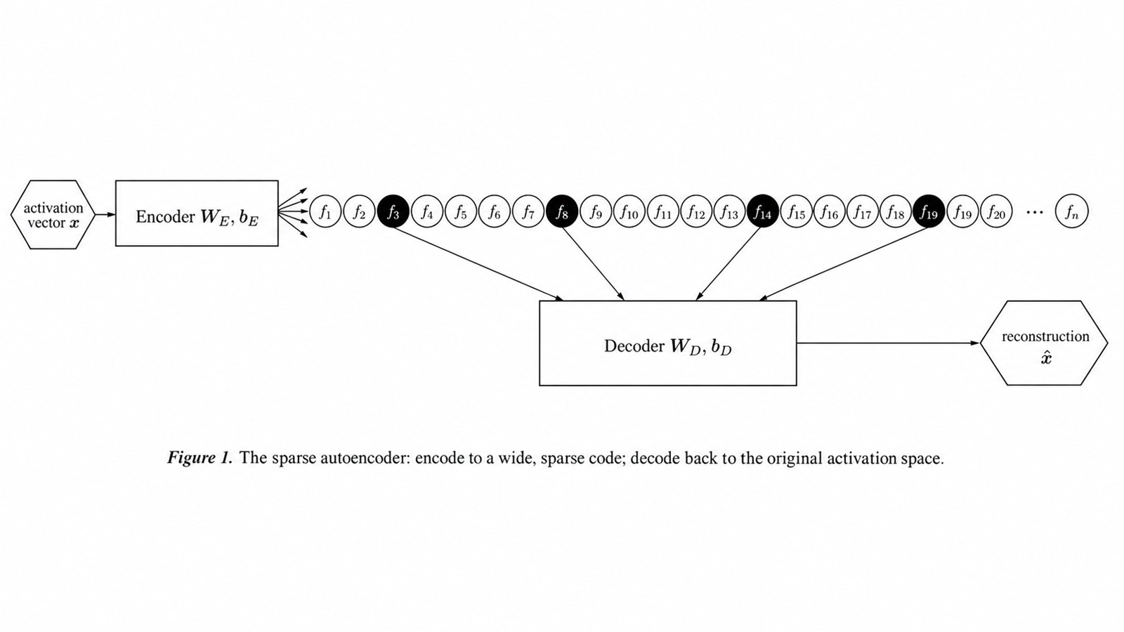
A standard sparse autoencoder maps an activation vector x (typically taken from a residual stream or MLP layer of the model being studied) through:

• An encoder: a linear projection into a much higher-dimensional space (the dictionary, often 8 to 64 times wider than the original activation dimension), followed by a nonlinearity that enforces sparsity, most commonly ReLU. This produces the sparse feature activations h.
• A decoder: a linear projection of h back down to the original activation dimension, producing a reconstruction x̂.

The training objective balances two competing terms: a reconstruction loss (how close x̂ is to x, usually squared error) and a sparsity penalty (typically an L1 penalty on h, though newer variants use different mechanisms, more on this below). The coefficient controlling the tradeoff between these two terms, usually written λ, is not a minor implementation detail. It is, as later sections will make explicit, the single dial that determines almost every downstream tradeoff this article covers.

1.2 Architectural variants, briefly

The field has moved through several generations of the same basic idea, each addressing a specific failure of the previous one:

• ReLU + L1 SAEs, the original approach. Simple, but the L1 penalty introduces a systematic bias (discussed in Section 5) and provides only indirect control over sparsity.
• TopK SAEs, instead of an L1 penalty, only the k largest activations are kept per input, with everything else zeroed. This gives direct, exact control over sparsity (L0 is fixed at k by construction) at the cost of a hard architectural constraint that doesn't adapt sparsity to how "easy" a given input is to reconstruct.
• BatchTopK SAEs, a refinement that enforces the sparsity budget as a batch-level average rather than a strict per-example constraint, allowing some inputs to use more active features than others while preserving the average.
• JumpReLU SAEs, use a learned, per-feature activation threshold instead of a fixed nonlinearity, aiming to combine the direct sparsity control of TopK-style approaches with more graceful handling of varying feature magnitudes.

Each of these has become a checkbox in the "we improved SAEs" literature, and each does measurably help with something. None eliminates the underlying tradeoffs this article walks through, they mostly reposition where on the tradeoff curve you land.

2. How an SAE Is Graded

Because there is no ground-truth list of "the true features a model uses," SAE quality is assessed through a small set of imperfect proxy metrics. Understanding what each one does and does not measure is a prerequisite for understanding why the tradeoffs in Section 4 onward are not fixable by simply "training a better SAE."

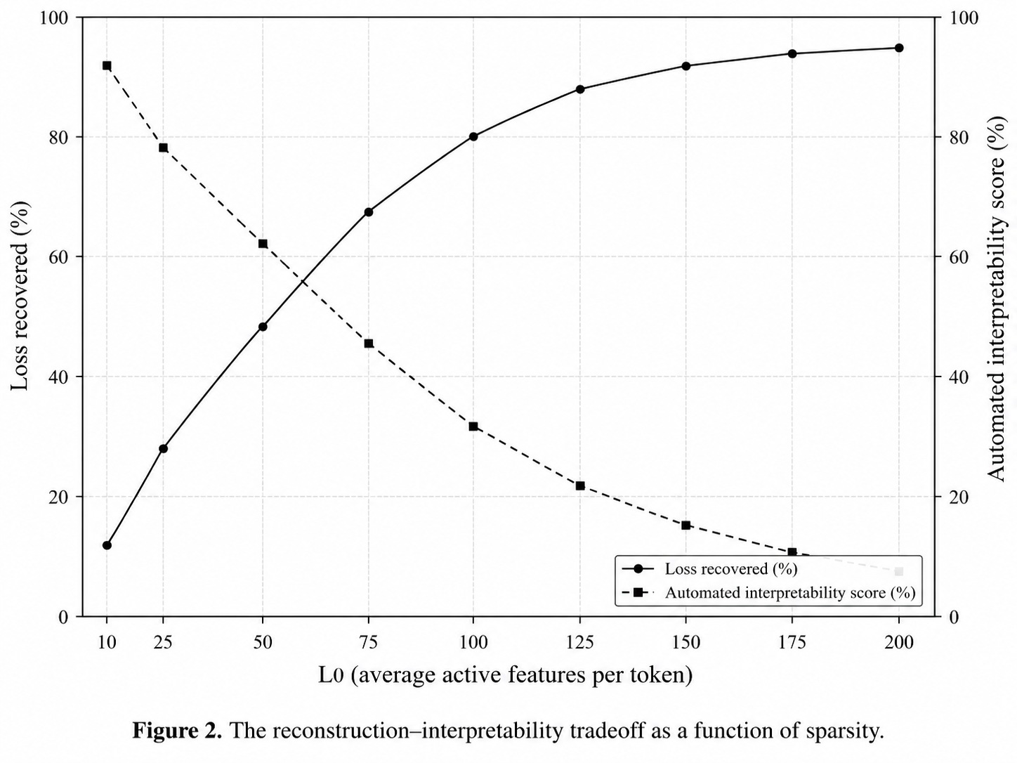
• L0 (sparsity), the average number of nonzero feature activations per input. Lower L0 generally correlates with easier-to-interpret individual features, because fewer things are "explaining" any given activation.
• Reconstruction error / normalized MSE, how far the decoded reconstruction x̂ is from the true activation x. This is a direct, easy-to-compute number, but it does not by itself tell you anything about whether the directions the SAE found are meaningful, a dense, uninterpretable code can achieve excellent reconstruction.
• Loss recovered, arguably the more decision-relevant metric: splice the SAE's reconstruction back into the model in place of the real activation, run the rest of the forward pass, and measure how much of the resulting increase in the model's loss (relative to leaving the activation untouched) is "recovered" relative to a naive baseline (such as replacing the activation with its dataset mean). A perfect SAE would recover 100% of the loss; in practice, this number is reliably less than 100%, and the gap is precisely the quantity Section 4 is about.
• Automated interpretability scores, since human labeling of thousands of features doesn't scale, the field relies on LLM-judged proxies. Two common ones are a detection score (can a held-out model, given a natural-language description of a feature, correctly identify which text snippets activate it?) and a fuzzing score (can it distinguish a feature's true activation pattern from a corrupted version?). These are useful and widely adopted, but they are themselves models grading models, with their own biases and blind spots, and they say nothing about whether a feature is causally important to model behavior, only whether its activation pattern is describable.

None of these four metrics move together. A change that improves one routinely degrades another. That is not a bug to be engineered away, it is the central fact of the whole field, and it is the subject of the rest of this article.

3. What SAEs Have Genuinely Revealed

Before the tradeoffs, it's worth being fair about what this method has actually delivered, because the tradeoffs are only interesting in the context of real, demonstrated value:

• Monosemantic features at meaningful scale. Anthropic's original 2023 demonstration (on a small one-layer transformer) and its 2024 follow-up (on the production-scale Claude 3 Sonnet) both found large numbers of features corresponding to specific, human-interpretable concepts, from concrete ones (a specific city, a chemical compound) to abstract ones (sycophancy, an internal sense of uncertainty, code security vulnerabilities), where the equivalent analysis performed directly on neurons had failed to find anything comparably clean.
• Causal steering. Because SAE features are (by construction) linear directions in activation space, clamping a feature's activation up or down and re-running the model lets you test, causally, whether that feature actually does what its label suggests. The well-known "Golden Gate Claude" demonstration, artificially amplifying a Golden Gate Bridge–related feature until the model became fixated on the bridge in almost every response, is exactly this kind of causal check, not just a pattern-matching exercise.
• A foundation for circuit-level analysis. SAE-style feature dictionaries (and their close relative, transcoders) are the substrate underlying circuit-tracing methodologies that connect features across layers into causal graphs describing how a model produces a specific output, work covered in depth in a companion piece to this article.
• Cross-domain transfer. The same basic recipe, train a sparse dictionary on a model's internal activations, has produced interpretable, biologically meaningful features when applied outside language models entirely, including protein language models and single-cell genomic foundation models, suggesting the superposition problem (and this proposed fix for it) is not specific to text.

This is genuine, replicated, causally-validated progress. It is also, on every one of the axes below, incomplete in ways that are easy to elide in a demo built around the features that worked.

4. The Central, Unavoidable Tradeoff: Sparsity vs. Fidelity

Here is the tradeoff that every other one in this article is a variation of, and the one most likely to be quietly left out of a headline result.

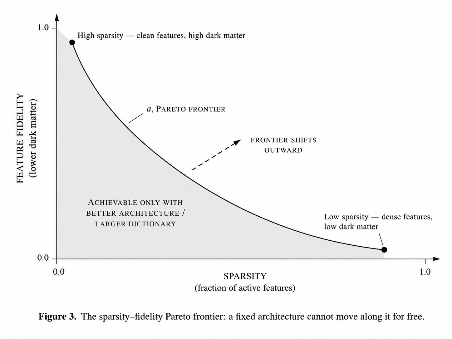
Sparser codes are more interpretable. Sparser codes are also less accurate. This is not an incidental finding, it follows directly from the training objective in Section 1.1, which literally weights these two things against each other. Pushing the sparsity penalty higher forces more features to zero, which does make each active feature's role easier to describe in isolation, but it also mechanically increases reconstruction error, because there is strictly less information being passed through to the decoder.

The unreconstructed remainder, the gap between the SAE's decoded output and the model's true activation, has been given a specific name in the literature: "dark matter." It is not simply small numerical noise. It represents portions of the model's actual computation that the SAE's feature dictionary, at its current size and sparsity level, has not learned to represent at all. Every downstream claim built on top of an SAE, a labeled feature, a causal steering result, a circuit-tracing edge, is implicitly a claim about the reconstructed portion of the model's computation, silently excluding whatever fraction lives in that unreconstructed remainder.

Two numbers make this concrete rather than abstract:

• Loss recovered figures reported across the literature routinely fall short of 100%, and the shortfall is not a rounding error, it represents real degradation in the model's actual next-token predictions when its true activations are swapped for the SAE's approximation. A "well-performing" SAE by current community standards is one whose loss-recovered figure is high, not one whose figure is perfect, perfect reconstruction essentially never happens at sparsity levels anyone considers interpretable.
• Comparative work explicitly plotting reconstruction error against automated interpretability score (the "reconstruction vs. interpretability curve," popularized in transcoder-comparison papers) shows this isn't a soft correlation, it's a genuine Pareto frontier. Improving one, at a fixed architecture and dictionary size, mechanically costs you the other. The only way to move the whole frontier outward, rather than just sliding along it, is a genuine methodological change (bigger dictionaries, better architectures, more training compute), not a hyperparameter tweak.

The practical implication, stated plainly: every SAE feature dictionary you look at was tuned to a specific point on this curve, and that point was a choice, not a discovery. A dictionary tuned for maximally clean, presentable features is, by the same training objective, a dictionary that is systematically worse at capturing the full range of what the model is actually doing, and a dictionary tuned to minimize reconstruction error will contain a meaningfully higher fraction of messy, hard-to-label, or polysemantic-again features. Papers and demos overwhelmingly show you the former.

5. Dead Features and Shrinkage: The Optimization Side Effects Nobody Puts on the Slide

Beyond the headline sparsity/fidelity tradeoff, the actual process of training an SAE introduces two well-documented optimization pathologies that further eat into the "real" capacity of the dictionary.

5.1 Dead features

A substantial fraction of the features in a trained dictionary can end up permanently inactive, never firing on any input in the training or evaluation distribution, contributing nothing to the model's understanding despite occupying a slot in the dictionary. Anthropic's own original research notes describe most features in very wide autoencoders ending up in an "ultralow density cluster," activating so rarely they are functionally dead for practical purposes.

This has a direct, quantifiable cost: a dictionary advertised as having, say, one million "features" may have a meaningfully smaller number of features that ever actually do anything on realistic inputs. Reported feature counts in papers and product marketing are dictionary sizes, not counts of features that meaningfully contribute to reconstruction.

The causes are now reasonably well characterized and split into (at least) two independent mechanisms:

• Geometric death at initialization, some features are simply born in a part of activation space they can never recover from, regardless of training dynamics.
• Training-dynamics death, even a death-free initialization can lose large fractions of its dictionary to dying features purely as an emergent consequence of the sparsity penalty during training; one study found dead-feature rates climbing to roughly 80% at high sparsity-penalty settings despite zero dead features at initialization.

Proposed mitigations, "ghost gradients" (an auxiliary loss term that gives dead features a gradient signal to recover), and mean-centering the input activations before encoding, each address one of the two mechanisms but not the other. Ghost gradients help with training-dynamics death but do little for geometric death; mean-centering fixes geometric death but does not address training-dynamics death. There is, as of this writing, no single fix that eliminates dead features across the board, only partial, mechanism-specific patches that need to be combined and still leave some dead-feature rate as a cost of doing business.

5.2 Shrinkage

A second, subtler pathology stems from the L1 sparsity penalty specifically (and, to varying degrees, its successors). Because an L1 penalty is proportional to the magnitude of active features, the optimizer is incentivized not only to make fewer features active, but to make the ones that are active smaller than their "true" magnitude would warrant, purely to reduce the penalty term, independent of whether that smaller magnitude actually reconstructs the input well. This systematic underestimation is called shrinkage, and Anthropic's own research notes explicitly attribute part of the gap between an SAE's achieved loss-recovered figure and what one might hope for to exactly this effect, rather than to fundamental capacity limits of the dictionary. Alternative penalty functions (such as a tanh-based penalty investigated in place of raw L1) have been explored specifically to reduce this bias, with partial success, again, a mitigation, not an elimination.

The upshot of this section: some meaningful fraction of any given SAE's measured shortfall from perfect reconstruction is not a fundamental limit of sparse coding as an idea, it is an artifact of specific, known quirks in how these networks are currently optimized. That is a more optimistic framing in one sense (these particular gaps may shrink with better training recipes) and a more damning one in another (it means published loss-recovered numbers conflate "fundamental capacity limit" with "current optimizer clumsiness," and readers generally have no way to tell how much of a given gap is which).

6. Feature Splitting and Absorption: The Dictionary-Size Problem

A separate and, in some ways, more conceptually troubling issue: the features an SAE finds are not stable with respect to dictionary size.

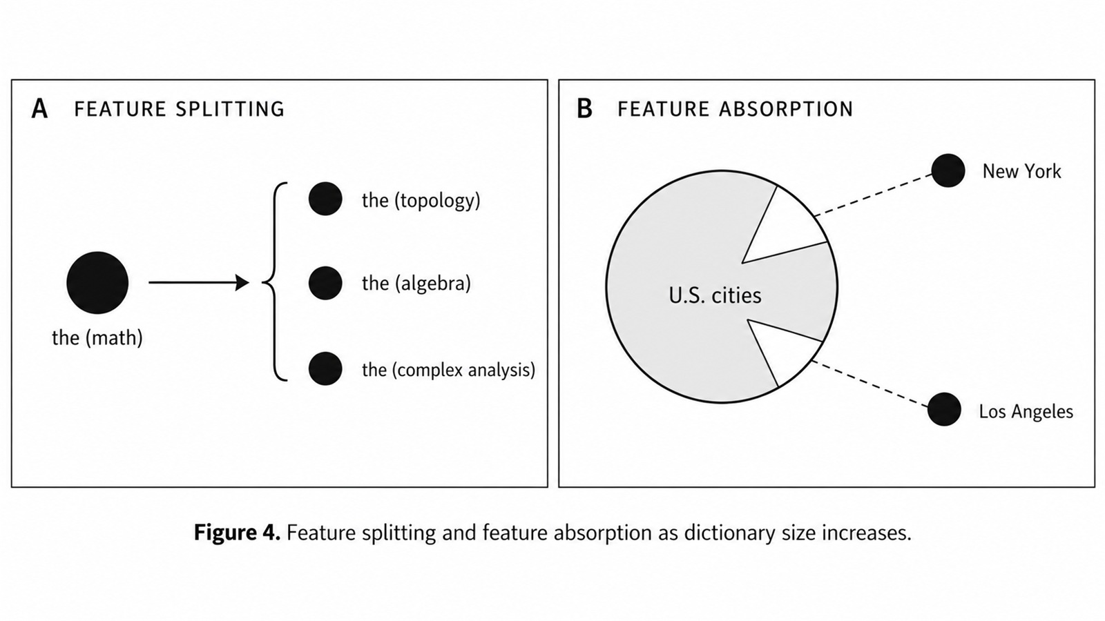
Feature splitting is the empirical observation that as you increase an SAE's dictionary size, a single, cleanly interpretable feature found by a smaller dictionary routinely fractures into multiple, more specific features in the larger one. Anthropic's own example: a feature representing "the word 'the' in mathematical prose," found by a smaller SAE, splits in a larger SAE into separate features for "'the' in topology and abstract algebra" versus "'the' in complex analysis," and further subdivisions beyond that. There are two live hypotheses for what this means, and they are not compatible with each other:

1. The maximally-split, most specific features are the model's real, "atomic" units, and the smaller SAE was simply too small to resolve them, it was conflating multiple true features into one, coarser feature out of necessity.
2. The atomic features are the coarser ones, and the split features found by larger SAEs are artificially manufactured composite features, the SAE is incentivized to create a single feature for two concepts that happen to frequently co-occur, because doing so is cheaper under the sparsity penalty than firing two separate atomic features every time, at the cost of slightly worse reconstruction.

These two hypotheses make opposite recommendations about which dictionary size to trust, and the field does not currently have a decisive way to adjudicate between them for a given feature.

Feature absorption is a related but distinct failure: a highly specific feature "steals" credit for a subset of cases that logically belong to a more general feature, leaving that general feature with unexplained gaps. The canonical illustrative example is a feature that behaves exactly like a general "U.S. cities" detector, except it mysteriously fails to fire for New York and Los Angeles, because those two cities have been absorbed into their own separate, more specific features elsewhere in the dictionary. A researcher looking only at the general feature would incorrectly conclude the model doesn't represent New York and Los Angeles as cities in this context, when in fact it does, just somewhere else in the dictionary, under a different feature ID.

Both problems get worse, not better, simply by training a bigger dictionary, bigger dictionaries reliably show more splitting and more opportunities for absorption, not less. Architectural proposals like Matryoshka SAEs (which train several nested dictionaries of increasing size simultaneously, structured so smaller sub-dictionaries are forced to capture general concepts on their own, without leaning on the larger dictionary's more specific features) are a direct response to this problem, and show measurable improvement, but they are a structural workaround for a symptom, not a resolution of the underlying question of what the "correct" dictionary size or feature granularity actually is.

7. Are SAE Features Even "Real" Units? The Canonicity Problem

A significant strand of recent research has directly tested, and cast doubt on, a foundational assumption implicit in most SAE-based work: that there exists a single, correct, "canonical" dictionary of atomic features a model uses, which an SAE trained at sufficient scale would eventually converge to.

Two specific experimental techniques were used to probe this:

• SAE stitching, take latents (features) from a larger, more expressive SAE and insert or swap them into a smaller SAE trained on the same model and data. Latents from the larger SAE separate cleanly into two categories: novel latents, which measurably improve the smaller SAE's performance when added, direct evidence the smaller dictionary was missing real information, i.e., was incomplete, and reconstruction latents, which can simply substitute for an existing latent in the smaller SAE without changing much. The existence of novel latents at every dictionary size tested is itself evidence against the idea that any given SAE, however large, has captured a complete feature set.
• Meta-SAEs, an SAE trained not on the underlying model's activations, but on the decoder matrix of another, already-trained SAE. If SAE features were truly atomic, a meta-SAE should find nothing further to decompose. Instead, meta-SAEs routinely decompose a single larger-SAE latent into a combination of several more primitive ones, the paper's example is a feature representing the specific person "Einstein" decomposing into more general constituent features for "scientist," "Germany," and "famous person." A feature that decomposes into other, more basic features under further sparse coding was not, definitionally, atomic in the first place.

Together, these results support a conclusion that is easy to state and somewhat uncomfortable for the field: *SAEs are not finding the features of a model. They are finding a set of features, at a particular scale and sparsity setting, that happens to be a locally reasonable, but neither unique nor complete, decomposition.* Different dictionary sizes and different training runs on the identical model and data can, and empirically do, surface meaningfully different feature sets, and there is no privileged size or seed you can point to as ground truth.

This is not a fringe finding; it directly informed follow-on architectural work (including the Matryoshka approach discussed above, and BatchTopK SAEs, introduced specifically to make meta-SAE training tractable) rather than being an isolated critique that the field simply ignored.

8. Instability: Same Model, Same Data, Different Features

A closely related and separately documented problem: SAEs trained on the same model, the same layer, and the same training data, differing only in random seed or minor hyperparameter choices, do not reliably converge to the same feature dictionary. This matters enormously for any claim of the form "the model has a feature for X," because that claim is implicitly a claim about a specific trained SAE artifact, not a directly verified property of the underlying model. A different research group, training their own SAE on the same publicly available model with slightly different settings, is not guaranteed to find the same feature, or to find it with the same clarity, cleanliness, or activation profile, and there is no established registry or canonical checkpoint that resolves disputes when two groups' SAE-derived claims about the same model disagree.

This instability compounds every other issue in this article rather than sitting alongside it: it means the sparsity/fidelity point you land on (Section 4), the dead-feature rate you get stuck with (Section 5), and the specific way splitting and absorption manifest (Section 6) are all, to a nontrivial degree, a function of decisions and randomness in a single training run, not fixed facts about the model being studied.

9. Interpretable Doesn't Mean Useful: A Second, Independent Axis

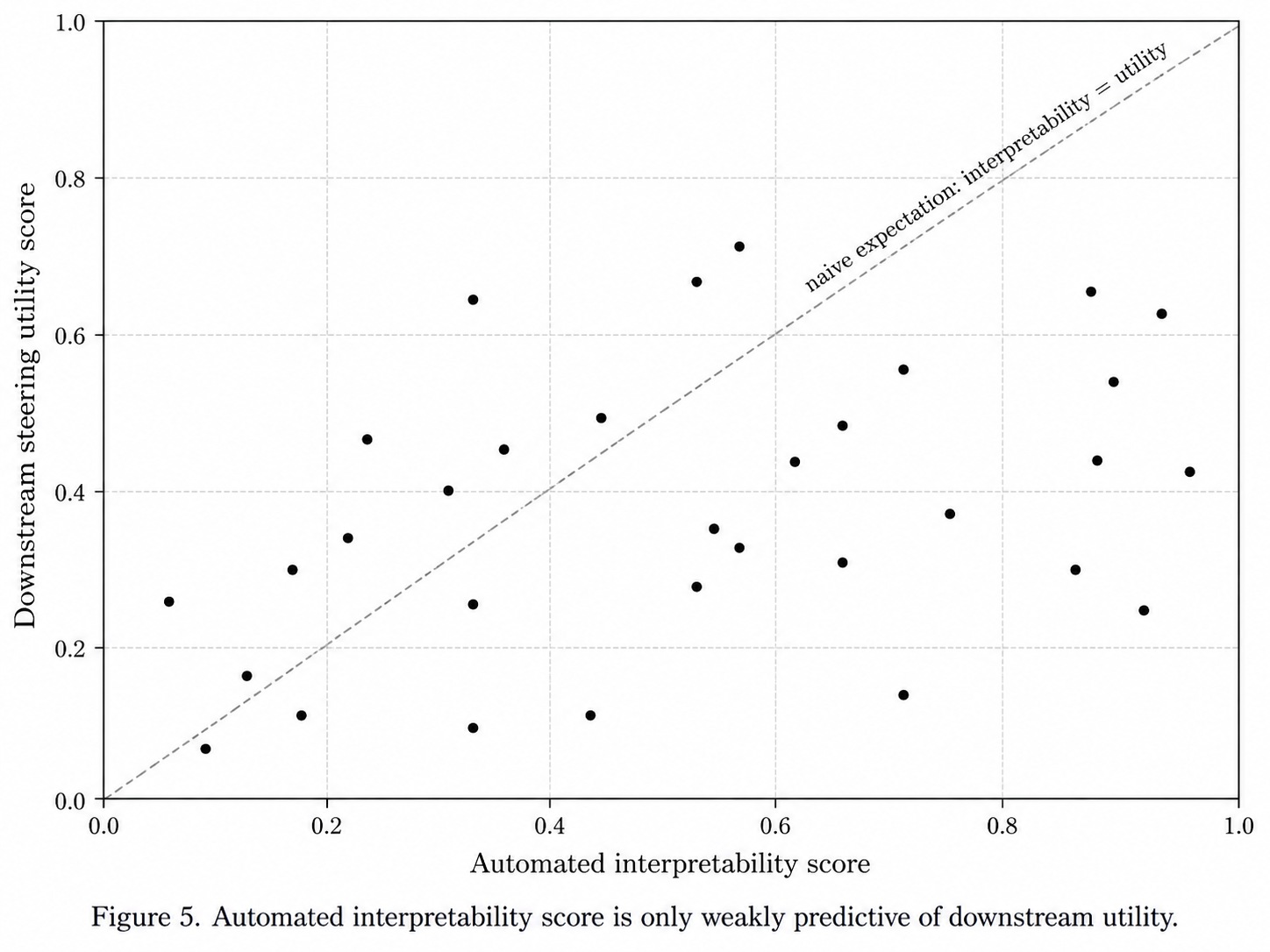
It is tempting to assume that if a feature scores well on automated interpretability metrics (Section 2), it must also be a useful unit for downstream tasks, steering the model, detecting a behavior, editing a concept out. Recent pairwise-comparison work has tested this assumption directly and found it does not reliably hold: interpretability score and downstream utility are, empirically, not the same axis, and a feature can score well on one while underperforming on the other.

This matters practically because most public-facing SAE work reports interpretability scores (because they're comparatively easy to compute and present well), while the harder, more decision-relevant question, "if I actually use this feature to do something, does it work as advertised?", receives comparatively less systematic evaluation. A feature dictionary optimized and marketed on the strength of its interpretability numbers is not automatically the same dictionary you'd want if your actual goal were reliable causal steering or robust behavior detection.

10. A Direct Competitor Exposes the Tradeoff Even More Starkly: Transcoders

Some of the clearest, most quantified evidence for the reconstruction/interpretability tradeoff comes from a body of work comparing SAEs directly against a close architectural relative: transcoders, which, instead of reconstructing a layer's own activations, are trained to reconstruct the output of an MLP block from its input (the same architectural family, incidentally, that underlies the cross-layer transcoders used in circuit-tracing methodology).

Head-to-head comparisons, holding model, data, and dictionary size fixed, found that transcoders produce measurably more interpretable features than SAEs at matched reconstruction performance, a genuine improvement on the tradeoff curve, not just a repositioning along it. A further architectural refinement, the "skip transcoder" (adding a direct affine skip connection alongside the sparse code), achieved lower reconstruction error still, with no measured cost to interpretability, a rare example of a change that shifts the Pareto frontier outward rather than trading one axis for the other.

The reason this belongs in an article about SAE tradeoffs, rather than being a footnote about a competing method, is what it implies retroactively about plain SAEs: if a closely related architecture can recover more of the "dark matter" at no interpretability cost, then a meaningful fraction of every published SAE's unreconstructed variance was not a fundamental limit of sparse coding as an idea, it was, at least in part, an avoidable cost of the specific architectural choice (autoencoding activations directly, rather than transcoding a computation), a distinction that is easy to lose when SAE results are presented as if reconstruction error were an intrinsic property of "how much of the model's superposition can be resolved" rather than a property of one specific implementation choice among several.

11. The Evaluation Problem Is Itself Unresolved

Step back and notice what all of Sections 4 through 10 have in common: every single tradeoff and failure mode described was identified using proxy metrics, loss recovered, automated interpretability scores, downstream task performance on hand-picked benchmarks, because there is no independent, ground-truth definition of "the features a model actually uses" to check any of this against directly.

This creates a genuine measurement circularity that the field is candid about but has not solved: automated interpretability scores are themselves computed by other language models, which have their own systematic quirks, and there is ongoing work specifically re-examining whether current evaluation protocols (built around cleanly monosemantic textbook examples) properly handle messier, more realistic cases, such as genuinely polysemous words, where "good" behavior for an interpretability metric is itself ambiguous to define. Benchmark suites (such as SAEBench) that aggregate multiple metrics into standardized comparisons are a meaningful step toward rigor, but aggregating several imperfect proxies into one suite does not manufacture the ground truth that was missing from each proxy individually, it mainly makes the tradeoffs more visible and comparable across papers, which is valuable, but distinct from resolving them.

The honest summary: the field can currently tell you, with reasonable confidence, that method A is better than method B on a specific, named metric, at a specific dictionary size, on a specific model and layer. It cannot currently tell you, in any metric-independent sense, how close any given SAE is to "the true features," because that phrase does not yet have an operational definition independent of the very proxies being used to evaluate it.

12. What This Costs Downstream, the Part That Doesn't Make the Slide

Pulling the previous eleven sections together into their practical consequence: every downstream application built on top of an SAE inherits its accuracy limitations, usually without restating them explicitly at the point of use.

• Feature-based demos (steering a model toward talking about a bridge, or suppressing a behavior by clamping a feature) work well specifically because they were built around features that happened to land on the favorable end of the tradeoff curve, cleanly interpretable, high-magnitude, low-dark-matter features. This is a real result, but it is also a selection effect: the same dictionary contains a comparable or larger number of features that are dead, split, absorbed, or otherwise messy, and a demo is under no obligation to show you those.
• Circuit-tracing and attribution-graph methods that chain features together into causal graphs are explicitly built on top of reconstruction-error "error nodes" that account for a real, non-trivial, and separately-quantified fraction of end-to-end causal paths, a direct, downstream consequence of exactly the dark-matter problem described in Section 4, inherited wholesale by any method that treats an SAE (or its transcoder cousin) as ground truth for what the model's computation looks like.
• Safety-relevant feature detection (finding a "deception" feature, a "harmful request" feature) inherits the instability problem from Section 8: a feature detector trained against one SAE run's specific dictionary is not guaranteed to generalize to a re-trained SAE on the same model, let alone to a different model, without re-validation, a nontrivial operational cost if such detectors were to be deployed as a monitoring layer rather than used purely for one-off research case studies.
• Cross-paper comparability is weaker than the shared terminology ("features," "monosemanticity," "interpretability score") suggests, because different papers routinely use different dictionary sizes, sparsity mechanisms, and evaluation protocols, any one of which can move a reported number substantially along the tradeoff curves described above. A claim that "SAEs found N interpretable features" in one paper and a similar claim in another are not necessarily measuring the same thing in the same way.

None of this is an argument that the method doesn't work. It is an argument that "works" is a claim relative to a specific, chosen point on a documented, unavoidable tradeoff curve, and that point is a design decision made by whoever trained the dictionary, not a fact discovered about the model.

13. Conclusion

Sparse autoencoders are a real methodological advance: they took a genuine, well-documented obstacle to interpretability, polysemantic neurons produced by superposition, and gave researchers a working, if imperfect, way around it, one that has produced causally-validated, individually checkable claims about what specific directions in a model's activation space represent and do. That is not a small achievement, and the case studies built on top of it (steering demonstrations, safety-relevant feature discovery, biological applications outside language models entirely) are genuine evidence the method captures something real.

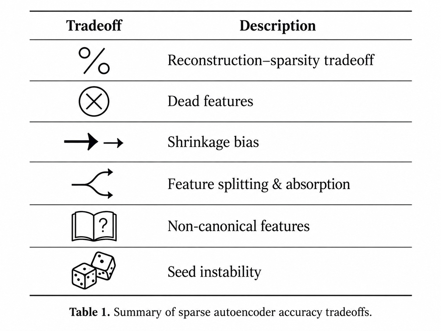
But "captures something real" and "captures everything, cleanly, in a stable and unique way" are very different claims, and the gap between them is not a minor asterisk, it is the specific, well-characterized, and actively-researched set of tradeoffs this article has walked through: a hard Pareto frontier between sparsity and fidelity that no fixed architecture escapes for free; dead features and shrinkage that quietly shrink a dictionary's effective capacity below its advertised size; feature splitting and absorption that make the "right" dictionary size an open question rather than a solved one; direct experimental evidence that SAE features are neither complete nor atomic; measured instability across nominally identical training runs; a documented gap between interpretability and downstream utility; a competing architecture that demonstrates some of the tradeoff was avoidable all along; and, underneath all of it, an evaluation framework built entirely on proxies because no ground truth exists to check against.

None of this is a secret, every claim in this article traces to a published paper, an official research note, or a direct architectural comparison. What is comparatively rare is seeing all of it assembled in one place, next to the demo, rather than scattered across limitations sections, appendices, and follow-up critiques that a casual reader of the headline result is unlikely to encounter.

Primary sources

• Bricken, Templeton, Batson, et al. (Anthropic), Towards Monosemanticity: Decomposing Language Models With Dictionary Learning, Transformer Circuits Thread, October 2023.
• Templeton, Conerly, Marcus, et al. (Anthropic), Scaling Monosemanticity: Extracting Interpretable Features from Claude 3 Sonnet, Transformer Circuits Thread, May 2024.
• Templeton, Batson, Henighan, Dying Features in Dictionary Learning, Circuits Updates, February 2024.
• Jermyn, Templeton, Batson, Bricken, Tanh Penalty in Dictionary Learning, Circuits Updates, February 2024.
• Leask, Bussmann, et al., Sparse Autoencoders Do Not Find Canonical Units of Analysis, ICLR 2025 / arXiv:2502.04878.
• Bussmann et al., Learning Multi-Level Features with Matryoshka Sparse Autoencoders, arXiv:2503.17547 (referenced via related work above).
• Minegishi, Furuta, Iwasawa, Matsuo, Rethinking Evaluation of Sparse Autoencoders Through the Representation of Polysemous Words, arXiv:2501.06254.
• Karvonen, Rager, Lin, et al., SAEBench: A Comprehensive Benchmark for Sparse Autoencoders in Language Model Interpretability, arXiv:2503.09532.
• Dunefsky et al., Transcoders Beat Sparse Autoencoders for Interpretability, arXiv:2501.18823, January 2025.
• Karvonen, An Intuitive Explanation of Sparse Autoencoders for LLM Interpretability, personal research blog, June 2024.
• Does Higher Interpretability Imply Better Utility? A Pairwise Analysis on Sparse Autoencoders, arXiv:2510.03659.
• On the Relationship Between Activation Outliers and Feature Death in Sparse Autoencoders, arXiv:2605.31518.
• Anthropic, Circuits Updates, July 2025, Transformer Circuits Thread (biological applications of SAEs).